GeoPandas: Plotting points with Point or MultiPoint geometry

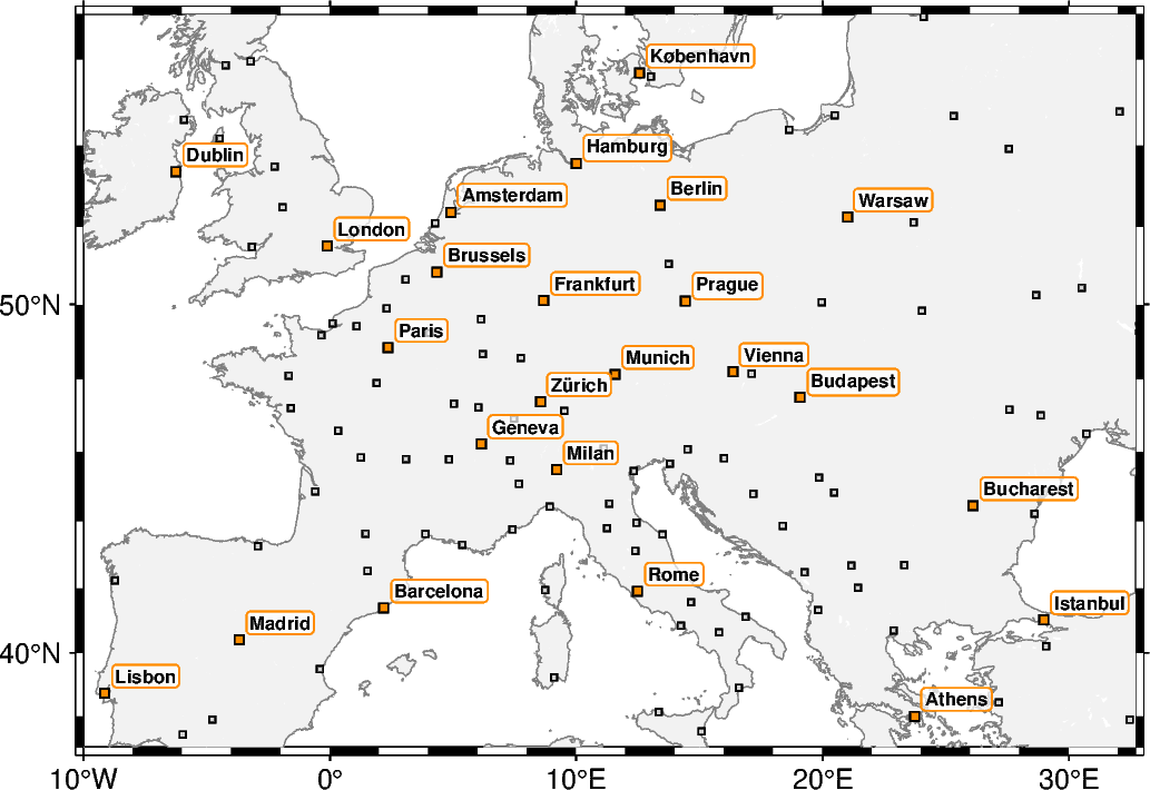
The pygmt.Figure.plot method allows us to plot geographical data such as points with Point or MultiPoint geometry types stored in a geopandas.GeoDataFrame object. Use geopandas.read_file to load data from any supported OGR format such as a shapefile (.shp), GeoJSON (.geojson), geopackage (.gpkg), etc. Then, pass the geopandas.GeoDataFrame object as an argument to the data parameter of pygmt.Figure.plot, and style the points using the fill and pen parameters. Additionally, pass suitable columns of the geopandas.GeoDataFrame to the x, y, and text parameters of the pygmt.Figure.text method to label specific features.

import geopandas as gpd
import pygmt

# Read a sample dataset provided by Natural Earth. The dataset contains cities stored
# as Point geometry type. In this example we focus on Europe.
provider = "https://naciscdn.org/naturalearth"
cities = gpd.read_file(f"{provider}/50m/cultural/ne_50m_populated_places_simple.zip")
cities = cities[cities["name"] != "Vatican City"].copy()  # No overlap with label Rome
# Create two subsets for small and large cities
cities_small = cities[cities["worldcity"] != 1].copy()
cities_large = cities[cities["worldcity"] == 1].copy()

fig = pygmt.Figure()
fig.basemap(region=[-10, 32.7, 37, 57], projection="M12c", frame=True)
fig.coast(land="gray95", shorelines="1/0.3p,gray50")

# Plot the two subsets using squares with different sizes and fills.
fig.plot(data=cities_small, style="s0.1c", fill="lightgray", pen="0.5p")
fig.plot(data=cities_large, style="s0.15c", fill="darkorange", pen="0.5p")

# Label the larger cities with their names.
fig.text(
    x=cities_large.geometry.x,
    y=cities_large.geometry.y,
    text=cities_large["name"],
    offset="0.12c",
    justify="BL",
    font="6p,Helvetica-Bold",
    fill="white@30",
    pen="0.5p,darkorange",
    clearance="0.05c+tO",
)

fig.show()